How to create conditional statements for drop-down lists in Google Sheets

If you fancy yourself a Google Sheets power user, have I got a tip for you. Have you ever wanted to create a spreadsheet that included the ability to select from a drop-down list, from which your selection would then dictate a value in another cell? This is called conditional statements and it’s an incredibly powerful tool that can make your spreadsheets far more accurate and user friendly.

For instance, say you had a list of services or products that you frequently sold to customers and clients. Each of those services or products had an associated and constant price. Instead of having to manually enter that price each time you create an invoice, you could simply select from a drop-down and your selection would then automatically populate another cell with the price.

Believe it or not, this is actually not too difficult. 

I want to show you how to create such a conditional statement.

SEE: Google Sheets: Tips every user should master (TechRepublic)

What you’ll need

The only thing you’ll need to make this work is a Google account. As long as you can log in to Google drive, you should be good to go.

How to create the drop-down list

The first thing we have to do is create the drop-down list, from which we’ll select our options. Let’s create a list with the following options:

• Blue with a value of 1

• Red with a value of 2

• Pink with a value of 3

• Purple with a value of 4

• Yellow with a value of 5

• Green with a value of 6

Of course, you use whatever you want for the “product” name as well as the value.

SEE: Hiring kit: Network administrator (TechRepublic Premium)

To create this drop-down, open a new Google Sheets document and select a cell. From the Data menu drop-down, select Data Validation (Figure A).

Figure A

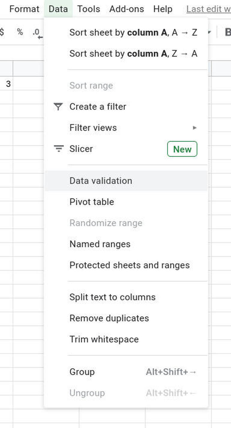
In the resulting window, you should see the cell you selected listed (Figure B).

Figure B

In the Criteria drop-down, select List Of Items. This will change the field to the right such that you can enter your items in a comma-separated list, so:

blue,red,pink,purple,yellow,green

Once you’ve entered the list of items, click Save and your drop-down is ready to go (Figure C).

Figure C

How to create the conditional statement

This is the more challenging part of the task, only because the conditional statement is a bit complex. 

Remember, we’re assigning numerical values to specific colors. The format of the conditional statement is:

=IF(CELL#="NAME",VALUE,IF(CELL#="NAME",VALUE,IF(CELL#="NAME",VALUE)))

Make sure you have as many right parenthesis as you have left, otherwise the statement will fail.

For our example, our drop-down is in cell A8, so the conditional statement would be:

=IF(A8="blue",1,IF(A8="red",2,IF(A8="pink",3,IF(A8="pink",4,IF(A8="purple",5,IF(A8="yellow",6,IF(A8="green,7)))))))

Once you’ve typed out the statement, hit Enter on your keyboard and it’s ready to go.

If you select a different entry from the drop-down, you’ll see the associated value populates the cell with the conditional statement.

That’s it, you’ve created a powerful tool to enhance your Google spreadsheets. Use this to give your spreadsheets more power and more accuracy.

Cloud and Everything as a Service Newsletter

This is your go-to resource for XaaS, AWS, Microsoft Azure, Google Cloud Platform, cloud engineering jobs, and cloud security news and tips. Delivered Mondays

Sign up today

Also see